1. Reports from Imperial College London

So far, Imperial College has published two reports on the early number of infections in the novel pneumonia outbreak in Wuhan: one on January 17 and another on January 22. Both estimate a population total from a sample, mainly using air-travel data and overseas cases to estimate the number of infections across Wuhan.

The English version of the calculation method in the official report:

English calculation method (redrawn from the text)

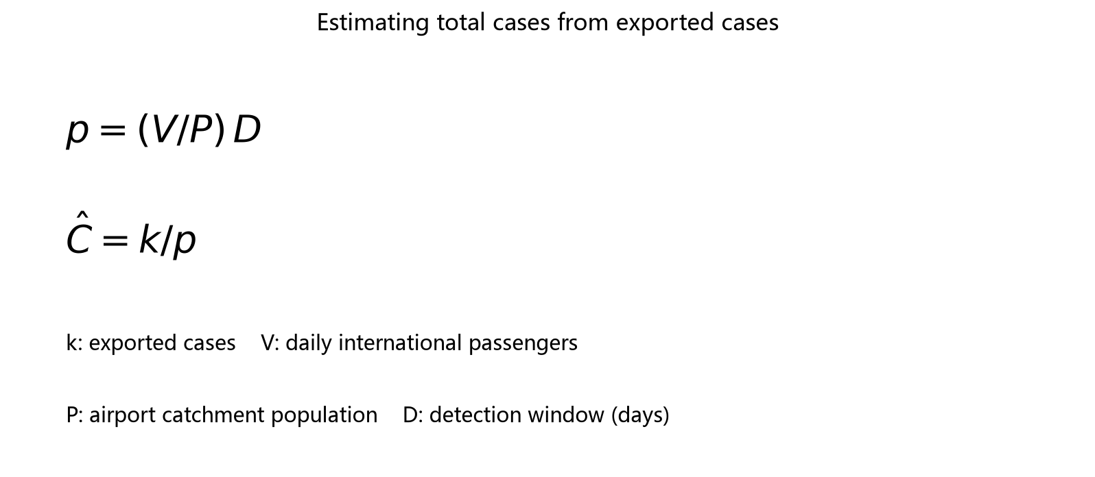
The second Imperial College report also included a Mandarin translation. The section below covers the calculation method.

Chinese calculation method (redrawn using the wording corrected in the article)

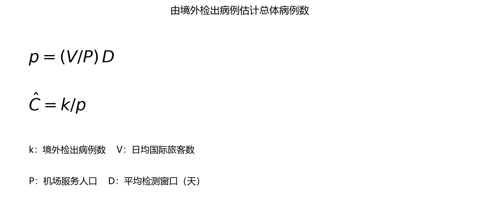
The Chinese translation is generally correct, but there is an error in the calculation of p. It translates this as p = probability of international travel per day x average probability of detecting one case. Based on the English and the model’s actual meaning, average probability of detecting one case should actually be the average time to detection, namely the detection window in the table (Detection window(days)).

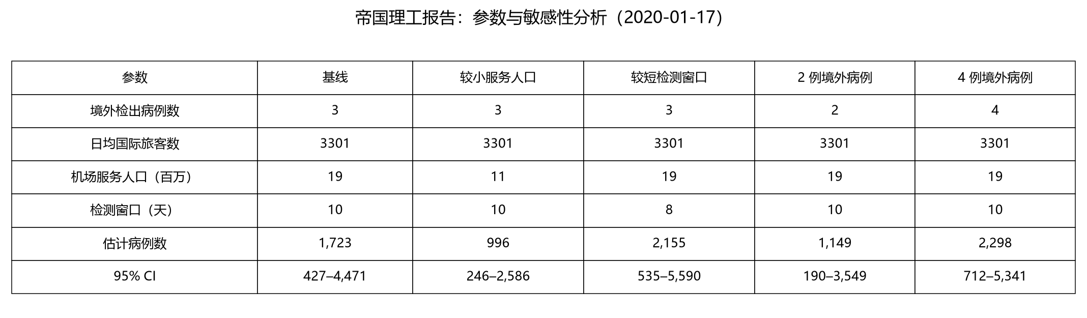
The first report uses data up to January 16. Taking the baseline as an example, the estimated total number of infections is 3/( (3301 / 1.9e7) * 10), approximately 1727. I am not sure why Imperial College used 1723, but the overall calculation method should be sound and the results are close.

2020-01-17 report parameter table (reformatted from the original report)

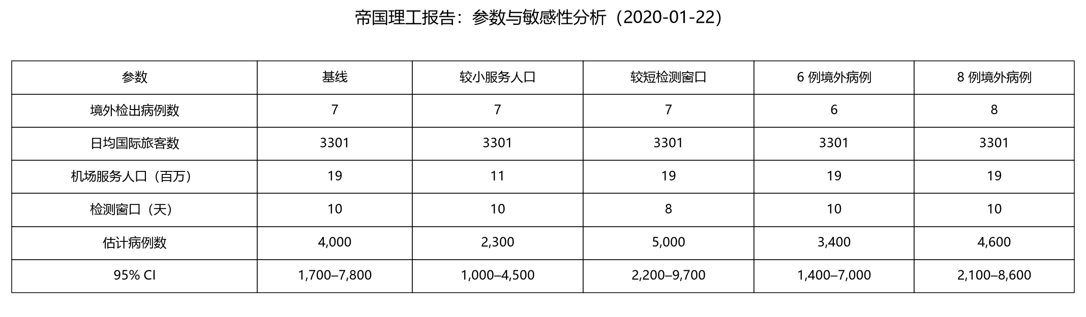
The second report uses data up to January 18. Confirmed cases abroad had risen to 7. Keeping the same method and parameters gives an estimated total of 7/((3301 / 1.9e7) * 10), approximately 4029.

Both reports also analyze sensitivity to the number of confirmed cases and the population effectively served by Wuhan International Airport, and calculate a 95% confidence interval for the possible range of estimated cases.

2020-01-22 report parameter table (reformatted from the original report)

Imperial College’s second report was released on January 22, while I am writing this article on January 17. More information has become available. First, there is information about the detection window, which the report defines as incubation period + time to confirmation. The report estimates an incubation period of 5–6 days, while the currently established figure (1/27) is an average of 10 days and a maximum of 14. This change would reduce the final result. Second, the population effectively served by Wuhan’s airport was estimated at 11–19 million. Recent news reports say around 5 million people left Wuhan before the lockdown and 9 million remained, totaling about 14 million—within that range.

Personally, I find the report’s result of 1700–7800 early infections credible because the model’s reasoning is reasonable and sound. One point I have not examined closely is the confidence-interval calculation, which I have not verified myself. Of course, the entire model rests on assumptions listed in the report, which are generally reasonable or have little effect on the final result.

The SIR Model

Another model I have seen in the media, besides Imperial College’s mathematical model, is SIR: an infectious-disease model based on differential equations. Details are shown below.

SIR model diagram (a reconstruction inferred from context)

SIR model curves (redrawn using the original parameters)

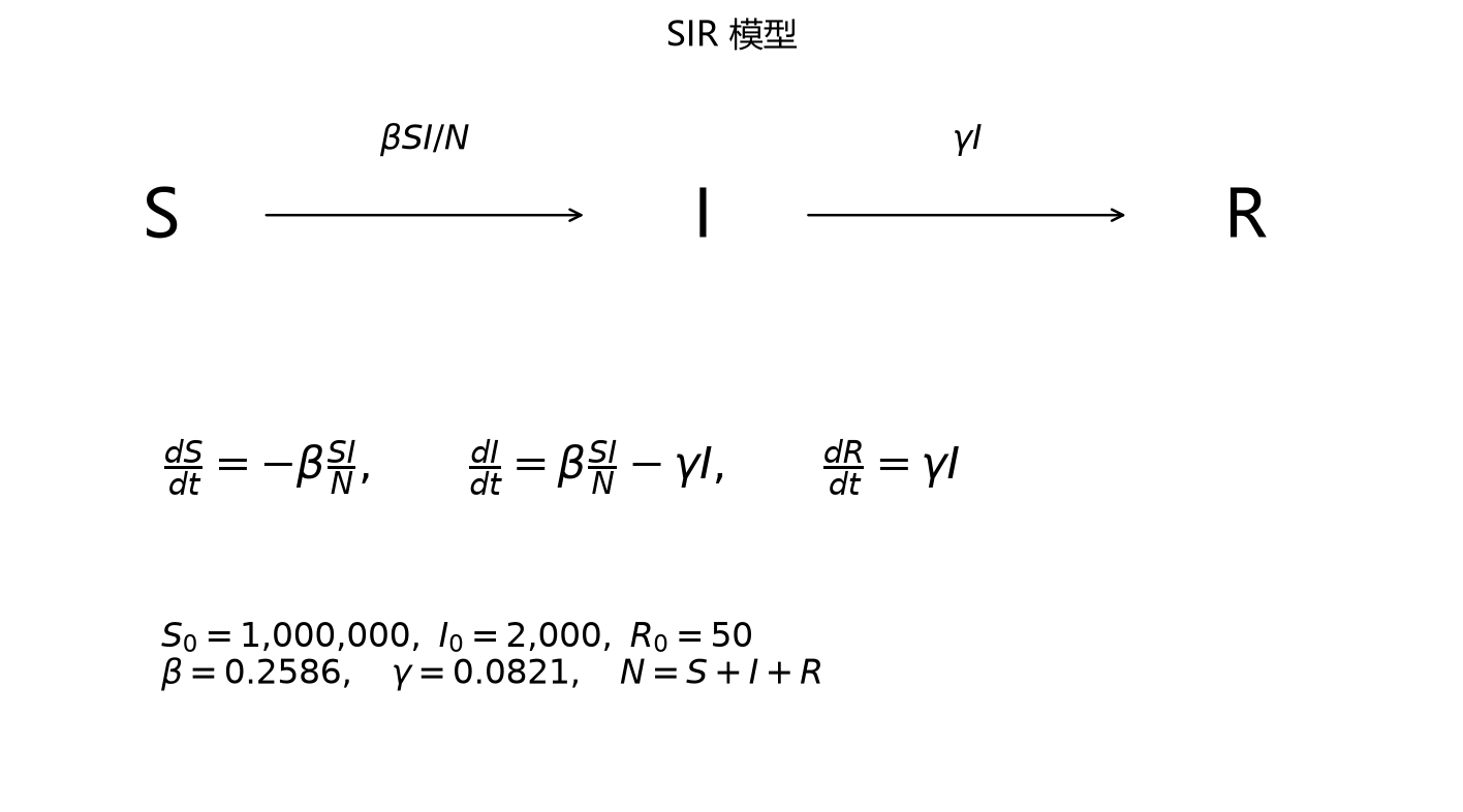
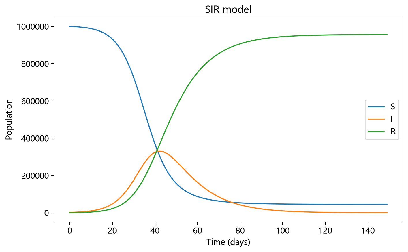
I was quite surprised when I first saw this model. Without using data from the current outbreak, it could largely match early developments and predict the epidemic’s course using parameters from the 2003 SARS model alone. That made me want to understand it. After looking at Baidu Baike, I felt that although the analysis and analytical solution might be difficult, repeatedly iterating to obtain a numerical solution and plot a similar graph looked straightforward. I decided to implement it in Python.

I initially used the equations from Baidu Baike, but the resulting graph was very strange. After repeatedly checking the code, I thought it was probably correct. Looking again at the graph above, I suspected it came from an interactive plotting page. Searching for the keywords “Hans Nesse - Gobal Health - SIR Model” quickly led me to the site: http://www.public.asu.edu/~hnesse/classes/sir.html. It also explained the differential equations below. Comparing these with Baidu Baike, I discovered that Baidu Baike had omitted the N in I*S/ N. After correcting the code and entering the same initial parameters as Professor Yu, it finally ran successfully. The code and result follow.

# 导入相关包
import numpy as np
import matplotlib.pyplot as plt

# 初始化参数
# 易感人群数量
S_0 = 0

# 初始感染数量
I_0 = 0

# 治愈和死亡数量
R_0 = 0

# 传染率beta
beta = 0

# 康复和死亡率
gamma = 0

# 德教授于晓华的参数
S_0 = 1000000
I_0 = 2000
R_0 = 50
beta = 0.2586
gamma = 0.0821

N = I_0 + S_0 + R_0


# 计算导数
def de_S(I, S):
    return -beta * I * S / N


def de_I(I, S):
    return beta * I * S / N - gamma * I


def de_R(I):
    return gamma * I


# 计算days天内的三种人数的数据

days = 150
X = np.arange(0, days)
# print(X)
I_t = np.zeros(days)
S_t = np.zeros(days)
R_t = np.zeros(days)

# 初始化
I_t[0] = I_0
S_t[0] = S_0
R_t[0] = R_0

for i in range(1, days):
    d_I = de_I(I_t[i - 1], S_t[i - 1])
    d_S = de_S(I_t[i - 1], S_t[i - 1])
    d_R = de_R(I_t[i - 1])
    I_t[i] = I_t[i - 1] + d_I
    S_t[i] = S_t[i - 1] + d_S
    R_t[i] = R_t[i - 1] + d_R


# 绘图
def plot():
    plt.plot(X, S_t, 'r--', X, I_t, 'b--', X, R_t, 'g--')
    plt.show()


plot()

SIR simulation results (redrawn from the original code)

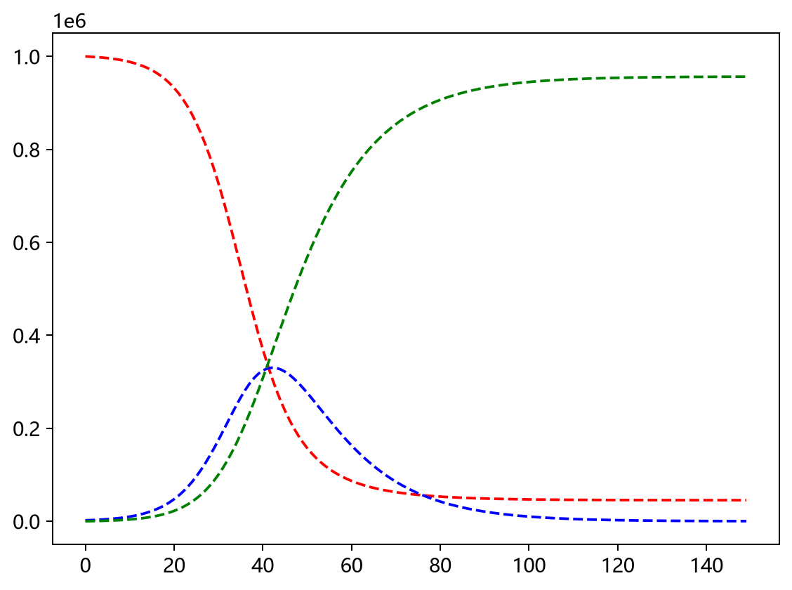
SIR is a basic infectious-disease model. In a closed environment, where S+I+R is constant, S is the susceptible population, I the infected population, and R the recovered population. A proportion of S becomes I after contact with I, and a proportion of I becomes R. S, I, and R change dynamically until they stabilize.

SIR does not otherwise use information about the outbreak: population, geography, early outbreak data, or measures such as isolation. All influences are reflected in the infection rate beta and removal rate gamma. There should be methods for estimating initial parameters from early outbreak data, but I have not explored that. Professor Yu also used SARS data. This outbreak differs from SARS: transmission can occur during incubation, it coincided with the Spring Festival travel rush in Wuhan, and the national response is different. Another point is that when the initial S is set to one million, I peaks at around 300,000. Most importantly, the model is too simple. So I do not find this SIR model very convincing.

Exponential Fitting Model

Neither model above uses the latest, most important data: the cumulative number of confirmed cases reported domestically each day. I think the population-growth “J” and “S” curves could be used for fitting. In the early phase of a novel coronavirus outbreak, growth is approximately exponential—a “J” curve—so an exponential function can fit it. As prevention and control measures, mainly isolation, take effect, the environment’s carrying capacity for the virus is constrained. Growth in confirmed cases slows and is eventually contained. Those confirmed cases then recover or die, and the epidemic eventually ends.

This mainly uses data from January 11 to January 26, from Wikipedia, because the sequence is continuous over that period. Earlier data are not only intermittent but fluctuate considerably. Also, adding the newly reported and confirmed cases does not quite match the final cumulative total. Since the discrepancy is small, I will not investigate it further here. The fitted curve and results are below:

Exponential fit (redrawn; results do not exactly match the original fit)

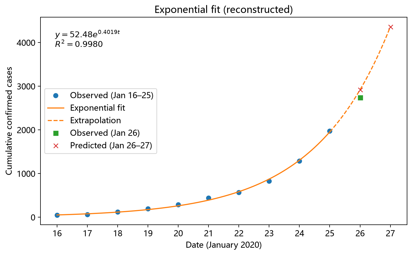
Here, data from January 16 to January 25 are used to fit the model and predict case counts for January 26 and January 27. The fitted curve has an R-squared of 0.99, indicating a very good fit. Although this does not mean the trend will continue indefinitely, it at least suggests that the epidemic is in its early outbreak phase and growing exponentially. The prediction for January 26 has an error of around 11%, which is already somewhat large. As for what happens next, we will have to wait for more data.